The Curious Landscape of Multiclass Learning

Posted On April 29, 2024

Welcome to the second installment of the Learning Theory Alliance blog post series! In case you missed the first installment on calibration, check it out here.

This time, Nataly Brukhim and Chirag Pabbaraju tell us about some exciting breakthrough results on multiclass PAC learning.

The gold standard of learning theory is the classical PAC model defined by Valiant in 1984 [Val84]. In particular, it allows us to reason about two fundamental questions: what can be learned, and how to learn it.

Generally in this setting, we are given some domain $\mathcal{X}$ (like images) and a label space $\mathcal{Y}$ (“dog” or “cat”?). The problem of learning a given class $\mathcal{H} \subseteq \mathcal{Y}^\mathcal{X}$ then boils down to finding a hypothesis $h \in \mathcal{H}$ after having observed training data drawn from some distribution $\mathcal{D}$ over $\mathcal{X}$ , such that $h$ has a small classification error with high probability, with respect to $\mathcal{D}$ .

For binary classification tasks, we get an especially clean and refined mathematical picture, in which these two questions are essentially resolved:

The question of what can be learned is answered via the Vapnik-Chervonenkis (VC) dimension [VC68, BEHW89], which completely characterizes learnability. A bit more concretely, the VC dimension is a combinatorial measure that quantifies the sample complexity needed to learn any given function class $\mathcal{H} \subseteq \{0,1\}^\mathcal{X}$ of binary classifiers.
The question of how to learn is resolved by a rich algorithmic and analytical toolbox. This includes, for example, the elegantly simple algorithmic principle of Empirical Risk Minimization (ERM), the clever boosting methodology, and sample compression scheme guarantees (we will elaborate more on these tools later on).

One might expect similar ideas to hold for multiclass classification tasks as well. After all, it is the most natural generalization of the binary setting to allow for more than two labels. Surprisingly, this is not at all the case! The story turns out to be much more complex and enigmatic when it comes to multiclass learning.

For example, the main question of what is learnable (i.e., extending the VC characterization of learnability) had been a longstanding open problem the study of which dates back to 1980s. Seminal works [NT88, Nat89, BDCHL95] identified that the Natarajan dimension characterizes PAC learnability when the number of classes is bounded. However, it remained unknown whether it also captures learnability when the number of classes is unbounded.

Similarly, the question of how also reveals a stark contrast between binary and multiclass classification.
One important example is the standard ERM principle which in fact fails to hold in the multiclass case [DSBDSS11]. Boosting theory also does not easily extend from the binary case [BHMS21, BDMM23], and it had been unknown whether learnable classes admit finite sized sample compression schemes in the multiclass setting, as is true in the binary one.

On the whole, the clean mathematical picture of binary classification did not generalize, revealing a landscape of multiclass learning far more puzzling than initially expected. In the past couple years, several advances were achieved, resolving some of these longstanding questions. In this post, we’re going to describe these results with the goal of demystifying multiclass learning and possibly shedding light on broader phenomena in learning theory.

The Question of What is Learnable and the DS Dimension

Many important machine learning tasks require classification into many target classes: in image object recognition, the number of classes is the number of possible objects. In language models, the number of classes scales with the dictionary size. In protein folding prediction, the goal is to predict the 3D structures of proteins based on their 1D amino sequence.

The fundamental question of what is learnable can be formalized as follows. For a domain $\mathcal{X}$ , and label space $\mathcal{Y}$ , we ask whether a given class $\mathcal{H} \subseteq \mathcal{Y}^\mathcal{X}$ is PAC learnable.

Definition (PAC learnability): We say that $\mathcal{H}$ is PAC learnable if there is a learning rule $\mathcal{A}$ for which the following holds. For any distribution $\mathcal{D}$ , target $h^\star \in \mathcal{H}$ , and $\epsilon,\delta > 0$ when given training set $S$ of ${{m}}_{ {\epsilon, \delta}}$ samples from ${\mathcal{D}}$ labeled by $h^\star$ , then the output of $\mathcal{A}(S)$ is a classifier $f_S: \mathcal{X} \rightarrow \mathcal{Y}$ that satisfies:

$\Pr_{S}\left[ \Pr_{x \sim \mathcal{D}}\left[ f_S(x) \ne h^\star(x)\right] \le \epsilon \right] \ge 1-\delta.$

The seminal result of Vapnik and Chervonenkis(1971) asserts that the finiteness of the VC dimension characterizes the sample complexity for the binary case, i.e., $|\mathcal{Y}| = 2$ . The VC dimension is a combinatorial measure of a the complexity of function class $\mathcal{H}$ . The definition of the VC dimension is not directly necessary to understand this blog post, but we state it here for the curious reader.

Definition (VC dimension): We say that $S \in \mathcal{X}^n$ is VC-shattered by $\mathcal{H} \subseteq \{0,1\}^\mathcal{X}$ if $\mathcal{H}|_S = \{0,1\}^n$ , where $\mathcal{H}|_S = \{h|_S : h \in \mathcal{H}\}$ ¹. The VC dimension $d_{VC}(\mathcal{H})$ is the maximum size of a VC-shattered sequence.

The characterization of learnability in the binary case is then given by the following tight bound on the sample complexity needed to PAC-learn any class $\mathcal{H}$ [Vap95, Han15]:

$m_{ \epsilon, \delta} = \Theta\left(\frac{d_\text{VC}(\mathcal{H}) + \log(1/\delta)}{\epsilon}\right).$

In the late 1980’s, Natarajan identified a natural generalization of the VC dimension. Later, [BDCHL95] showed that it exhibits the following bounds:

$C_1 \left(\frac{d_\text{N}(\mathcal{H}) + \log(\frac{1}{\delta})}{\epsilon}\right) \le {{m}}_{ {\epsilon, \delta}} \le C_2 \left(\frac{d_\text{N}(\mathcal{H})\log(|\mathcal{Y}|) \log(\frac{1}{\epsilon}) + \log(\frac{1}{\delta})}{\epsilon}\right),$

where $C_1,C_2 >0$ are absolute constants, and $d_N$ is the Natarajan dimension. Notice that the Natarajan dimension exhibits similar bounds to the binary case, up to a factor of $\log(|\mathcal{Y}|)$ . However, this factor can be huge or possibly infinite for tasks that do not admit an a priori reasonable bound on the number of classes, rendering the existing Natarajan-based bounds vacuous. It is therefore a natural question to ask whether we can get rid of the $\log(|\mathcal{Y}|)$ factor?

In 2014, Daniely and Shalev-Shwartz [DSS14] studied general algorithmic principles of the multiclass setting. Their analysis led them to identify a new notion of dimension, later named the DS dimension. Initially, they proved that a finite DS dimension is a necessary condition for PAC learnability, as is true for Natarajan dimension. They then conjectured that a finite DS dimension is also a sufficient condition, but they too left the full characterization of learnability open.

The answer finally arrived in 2022, when [BCDMY22] showed that the DS dimension is indeed the correct characterization for multiclass learnability.

We will now introduce the DS dimension. Two useful concepts that we will need are the notions of a one-inclusion graph and a pseudo-cube. The idea here is to translate a learning problem
to the language of graph theory. For any $n > 0$ and set $H\subseteq \mathcal{Y}^n$ , the one-inclusion graph of $H$ is a hypergraph $\mathcal{G}(H)=(V,E)$ that is defined as follows. The vertex-set is simply $V=H$ . For the edge set, we have that two nodes are connected by an edge when they differ in their labeling of exactly one coordinate.

Then, an $n$ -pseudo-cube is a finite set of vectors $H \subseteq \mathcal{Y}^n$ such that for every $h \in H$ and $i \le n$ there is $h' \in H$ that agrees with $h$ on all coordinates but $i$ . It can also be viewed as a finite subset of a one-inclusion graph on $H \subseteq \mathcal{Y}^n$ with edges on all coordinates.

Notice that when $\mathcal{Y} = \{0,1\}$ , the two notions “boolean cube” and “pseudo-cube” coincide, but when $\lvert \mathcal{Y}\rvert >2$ , that is no longer the case. Intuitively, a pseudo-cube can be thought of as a generalization of the boolean cube, where every element in the pseudo-cube $H$ has a “neighbor” on every coordinate.

As a simple example, let’s say the domain $\mathcal{X}$ is of size $2$ , and assume we have $3$ labels: $\mathcal{Y} = \{0,1,2\}$ . We can represent any class $\mathcal{H}$ by a graph, where each node corresponds to some $h \in \mathcal{H}$ . Each edge is colored to denote which coordinate changes:

The above graph is an example of a $2$ -pseudo-cube corresponding to a set $H$ of six $2$ -dimensional vectors. If any of these were removed, the remaining set $H' \subsetneq H$ would no longer form a pseudo-cube since it will violate the definition above.

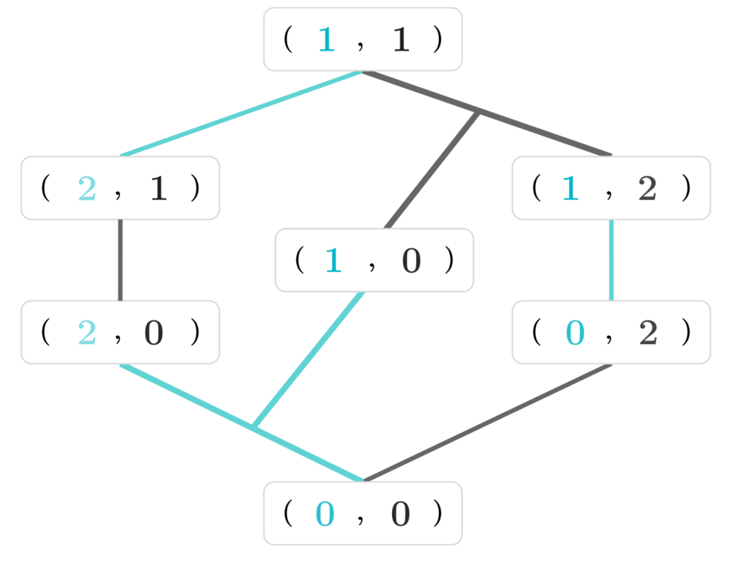
Alternatively, if another $2$ -dimensional vector was added, say $(1, 0)$ , the new set would also form a $2$ -pseudo-cube since each element (or node) in the new set also has a “neighbor” on every coordinate. Notice that this time we also have hyper-edges that contain more than $2$ nodes.

We are now ready to define the DS dimension. We say that $S \in \mathcal{X}^n$ is DS-shattered by $\mathcal{H}\subseteq \mathcal{Y}^\mathcal{X}$ if $\mathcal{H}|_S$ contains an $n$ -dimensional pseudo-cube. The DS dimension $d_{DS}(\mathcal{H})$ is the maximum size of a DS-shattered set.

Multiclass Characterization

The result showing that the DS dimension indeed characterizes learnability gives the following upper bound on the sample complexity [BCDMY22]:

${{m}}_{ {\epsilon, \delta}} = \Tilde{O}\left(\frac{d_{DS}^{1.5}}{\epsilon}\right),$

where $d_{DS}$ is the DS dimension of the class. Combined the previously known lower bound [DSS14] of $\Tilde{\Omega}\left(\frac{d_{DS}}{\epsilon}\right)$ , we get the complete characterization of the multiclass sample complexity.

The proof of the upper bound above involves many components and uses a variety of classic algorithmic ideas such as boosting, sample compression, transductive learning, ERM, and shifting. In addition to these classic tools, the proof also relies on resolving a new intermediate learning problem, which is interesting in its own right: namely, a setting where instead of predicting a single label for a given input, the goal is to provide a short list of predictions. The setting is called “list PAC learning”.

Intuitively, list-learning extends the standard PAC model by allowing the learning algorithm more freedom, and is a useful relaxation of the problem. One can also easily imagine scenarios where list-learning is itself a practical goal. For example, it can offer physicians a list of likely diagnoses, it can provide businesses the list of consumers’ preferences, and so on. This new setting has been since studied in several subsequent works [CP23, MSTY23]. Next, we’ll see how list-learning is a key step towards proving our desired bound.

The starting point of the proof is a combinatorial abstraction of the learning problem by translating it into the language of hypergraph theory. This results in algorithmic problems on the objects referred to as “one-inclusion graphs”, that we defined earlier. The one-inclusion graph leads to a simple but useful toy model for transduction in machine learning.

The toy model is as follows. Imagine a learning game played over a one-inclusion graph $(V, E)$ . The input to the problem is an edge. The input edge $e$ is generated by first fixing some node $v^*$ , and then choosing $e$ to be a uniformly random edge containing $v^*$ . The goal is to output a vertex $u$ that is equal to $v^*$ with as high probability as possible.

Now, notice that learning algorithms in this toy model are in fact orientations of the graph. Let’s see a simple example. Consider the following one-inclusion graph, similar to the ones we saw above (but is not a pseudo-cube):

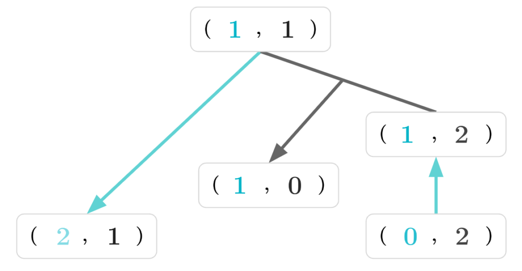
Observe that we simply oriented the edges of the graph, by choosing a single “representative” for each edge, to which it points to. An orientation is equivalent to a learning algorithm in the toy model, since it tells us which node to predict. Let’s assume that we chose $v^*$ to be the node $(1,2)$ . Then the pictured orientation would make a mistake if given the darker edge, and be correct if given the brighter edge.

Intuitively, the more edges that are oriented outwards of a node – the more mistakes the learner will make if that node were the chosen $v^*$ . Therefore, a useful observation here is that bounding the error of the learner corresponds to bounding the largest out-degree of the orientation. That way, we guarantee that no matter which $v^*$ was chosen, the worst case error is at most the maximal out-degree.

But how does that toy model relate to our original problem? We can think of an input edge as revealing the values of all coordinates, or data points, labeled by the “ground truth” node $v^*$ . Given values for all coordinates except one, we will try to predict it, which is equivalent to our test point. Then, by simple symmetrization arguments, “good orientations” of the one-inclusion graph can actually be shown to yield non-trivial learning algorithms for our original task.

So, we now want to solve the simpler problem of finding a good orientation for the one-inclusion graph $(V, E)$ induces by our hypothesis class $H$ . Recall that we assume the class has a bounded DS dimension $d_{DS} < \infty$ . Based on the properties of the DS dimension, it turns out that we can actually construct a good orientation with a maximal out-degree that is at most ${d_{DS}}$ .

Translating this orientation back to our original problem, we get a (very) weak learner which has error of $1-\frac{1}{d_{DS}+1}$ . This error is pretty high, but the crucial point is that it is uniformly bounded away from $1$ . So we managed to get a non-trivial error, but it is not clear how to proceed. How can we improve it?

It may be tempting to try to improve the error by boosting. But standard boosting turns out to be useless in our context, since the error is so high.

It is at this point that list learning comes to the rescue. We can show that the very-weak learner actually yields a list-learner where the list is of size $\approx d_{DS}$ . Then, the idea is to “map” each point $x \in X$ to a short list of labels, which allows us to eliminate the vast majority of a priori possible labels. Instead of all of $\mathcal{Y}$ , we can safely use the learned list $\mu(x)$ as the effective “local” label space for $x$ . Therefore, lists can be thought of as tools for alphabet reduction.

To conclude the proof, it is natural to try to reduce the learning task to one in which the number of labels is bounded. But, did we just reduce the infinite alphabet case to the finite case? The short answer is no, since the class restricted to our learned list may not contain the target function and may even be vacuously empty. The solution instead is based on learning algorithms that operate on the one-inclusion graph, and have a “local” property which is able to avoid the problem we raised.

The full algorithm is best thought of as a sample compression scheme, which demonstrates that a small subsample of the training data suffices to determine a hypothesis that correctly classifies all examples in it. We elaborate more on sample compression scheme later in this blog post.

Thus, we conclude the high-level outline of the proof for the upper bound on sample complexity via the DS dimension. While this proof is intricate, containing many details and components that are beyond the scope of this post, we hope that this overview captures the main ideas and sparks your interest in exploring the paper further.

DS Dimension vs. Natarajan Dimension

So we saw that the DS dimension characterizes multiclass learnability. But what about the Natarajan dimension, which had been the leading candidate to be the correct answer since the 1990’s?
Could it be essentially equivalent to the DS dimension? Perhaps it scales with the DS dimension up to certain factors?

The answer is no! The work by [BCDMY22] shows an arbitrarily large gap between the DS and the Natarajan dimension, proving that the Natarajan dimension in fact does not characterize learnability in the general case.

To understand this result, we first define the Natarajan dimension. We say that $S \in \mathcal{X}^n$ is N-shattered by $\mathcal{H} \subseteq \mathcal{Y}^\mathcal{X}$ if it contains an $n$ -Natarajan cube. A set $H \subseteq \mathcal{Y}^n$ is an $n$ -Natarajan cube if for every $i \in [n]$ there exists $a_i,b_i \in \mathcal{Y}$ , $a_i \ne b_i$ , and it holds that $H = \Pi_{i=1}^n \{a_i,b_i\}$ . The Natarajan dimension $d_{N}(\mathcal{H})$ is the maximum size of an N-shattered sequence.

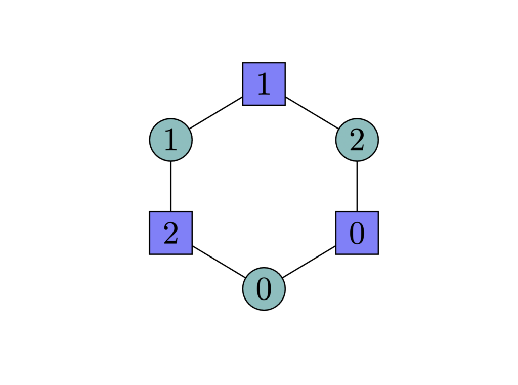
Let’s look at a simple example of a domain $\mathcal{X}$ of size $2$ , and label space $\mathcal{Y} = \{0,1,2\}$ . We can see that the Natarajan cube is a simple generalization of the boolean cube:

It may help to notice that the 2-Natarajan cube is equivalent to containing a square as a sub-graph of the corresponding one-inclusion graph. This intuition will help explain the separation result for higher dimensions. Let’s start with the simplest case we can show between the Natarajan and DS dimensions: $1$ vs. $2$ . In fact, we already saw it before:

Here, as we said earlier, the DS dimension is 2. But the Natarajan dimension is only 1. Intuitively this can be seen by the fact that there is no sub-graph that is a square.

And what about a larger separation? How large can this gap be?

Before we continue, we introduce a connection between learning and topology. It turns out that there is an interesting equivalence between hypothesis classes $\mathcal{H} \subseteq \mathcal{Y}^n$ and topological objects called “colored simplicial complexes”, which are combinatorial abstractions of triangulations of topological spaces. Let’s see our previous example, now by a colored simplicial complex:

In 2 dimensions, a simplicial complex is simply a graph. Here, each node correspond to a certain label, at a certain position. The circle node appears as the first symbol, and the square appears as the second symbol. There is an edge between two nodes if they correspond to a “word”, a hypothesis in $\mathcal{H}$ .

Importantly, it can be shown that a 2-Natarajan cube also corresponds to an embedded square in a simplicial complex. So, we can see that the above simplicial complex does not have a square as a sub-graph and therefore, we get that 1 vs. 2 separation as we said. That is, the DS dimension is 2 but the Natarajan dimension is only 1.

Now let’s try to get a separation of 1 vs. 3.

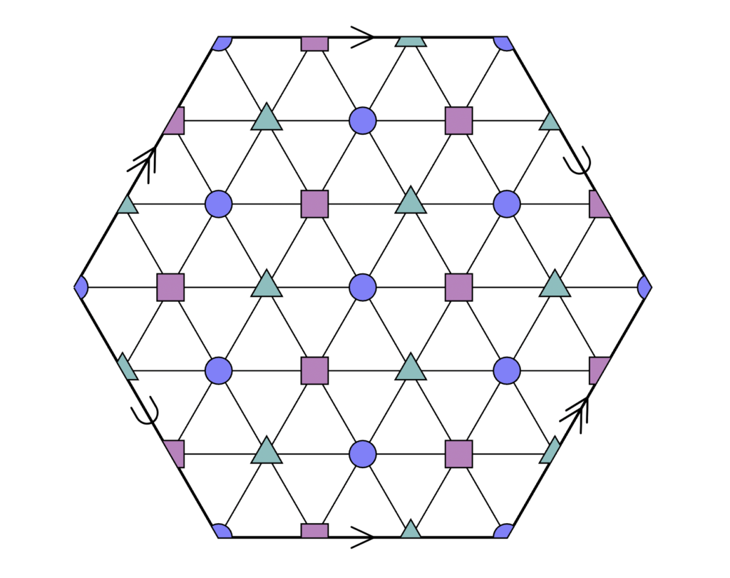
This is an example of a 3-dimensional pseudo-cube with Natarajan dimension 1. The “elements” in this larger pseudo-cube are the triangles (there are 54 of them). Each such triangle corresponds to a “word”, a hypothesis in $\mathcal{H}$ , over 3 coordinates. The labels are the vertices (there are $\tfrac{3 \cdot 54}{6} = 27$ of them). The vertices are colored by 3 colors: circle-blue, triangle-green and square-pink. In each word, the circle-blue vertex appears as the first symbol, the triangle-green vertex as the second, and the square-pink vertex as the third. Opposite sides of the hexagon are identified, as the picture indicates. The pseudo-cube property holds because each triangle has three neighboring triangles that are obtained by switching one vertex from each color. The Natarajan dimension is 1 because, again, there is no square (a cycle of length four) in the graph so that its vertices have alternating colors.

Notice that in this example, the complexity here increased pretty quickly – we only needed 6 elements to prove a gap of 1-to-2, and for 1-to-3 we already need 54. What about 1-to-4? This is much more difficult. A computer search found such a gap 1-to-4, corresponding to a class of size 118098! Should we give up on a systematic way to find a larger gap?

Let’s go back to the connection we mentioned between learning and topology. Interestingly, this equivalence turned out to be a lot richer than it initially seemed to be. In particular, notions similar to our dimensions have also been studied in algebraic topology. A Natarajan dimension of 1 corresponds to a local combinatorial criteria for hyperbolicity. A DS dimension of $d$ corresponds to the notion of a pseudo-manifold.

Building on this unique and beautiful connection, and using a deep and involved result in algebraic topology by Januszkiewicz and Świątkowski, 2003, it was proved in [BCDMY22] that the gap can be unbounded! That is, there exists a class with infinite DS dimension, but a Natarajan dimension of 1.

The Question of How to Learn

The VC/DS dimensions characterize what classes can be PAC learned. But how does one learn these classes? In the binary classification setting, a variety of tools including Empirical Risk Minimization (ERM), boosting, as well as sample compression schemes, each yield successful learning algorithms. As it turns out, each of these tools end up having some deficiencies in terms of how they extend to the multiclass setting.

Empirical Risk Minimization and Uniform Convergence

Finite VC dimension in the binary classification setting, which is a necessary condition for PAC learning, also endows a hypothesis class with a very special property — that of uniform convergence. Uniform convergence guarantees that the empirical loss of every hypothesis in the class on a sufficiently large (but finite) sample is close to its population loss with respect to the entire distribution. Because of this, the ERM algorithm, which simply outputs any hypothesis in the class that minimizes the error on the training dataset, is a valid learning algorithm.

In the setting of multiclass learning, if the Natarajan dimension of the class as well as the number of labels is finite, then the class still satisfies uniform convergence. However, the situation drastically changes when we allow an unbounded number of labels. In this case, it is possible to construct learnable hypothesis classes, which do not satisfy uniform convergence, meaning that for these classes, two different hypotheses from the class that each minimize the empirical risk could differ by an arbitrarily large factor in their population risk [DSBDSS11]! Thus, we can no longer always rely on the ERM principle for learning in the multiclass setting.

Boosting

Another common approach to obtain a PAC learner is via boosting. Namely, in the binary setting, having a weak learner that simply has error bounded away from $\frac12$ (i.e., better than random guessing) is sufficient to obtain a learner that has error $\epsilon$ (namely, a strong learner), via algorithms like AdaBoost [Fre95]. If the learning task is instead over $k$ labels, we could imagine that having a classifier that does slightly better than random guessing, i.e., has error slightly better than $1-\frac1k$ , would similarly allow us to obtain a strong learner via boosting. However, such a learner turns out to be too weak in order to plug into standard boosting algorithms [Chapter 10 in SF12, BHMS21, BHM23 , BDMM23]. Essentially, one still ends up requiring a weak learner with error below $\frac12$ , which is harder to obtain as $k$ gets large. Therefore, boosting too does not seem to give us a PAC learner in the multiclass setting, at least in a straightforward way.

Sample Compression

Finally, another standard way to obtain a learner is via sample compression. Roughly speaking, a hypothesis class admits a sample compression scheme, if for every sample labeled by a hypothesis from the class, it is possible to retain only a small subsample, using which the labels on the entire sample can be inferred. As a standard example, consider the binary hypothesis class of axis-aligned rectangles in two dimensions. Suppose we are given a training dataset labeled by some unknown rectangle, as in the figure below.

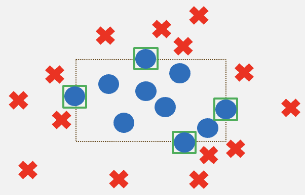
Observe how we can get rid of all samples except the left-most, right-most, top-most and the bottom-most circle, and simply draw a rectangle with these four points determining the boundary — this correctly classifies all the points, including the ones we threw away.

More concretely, a sample compression $(\kappa, \rho)$ for a hypothesis class $\mathcal{H}$ comprises of:

A compressor $\kappa:$ $\underbrace{(\mathcal{X} \times \mathcal{Y})^*}_{\text{training sample}} \to \underbrace{(\mathcal{X} \times \mathcal{Y})^*.}_{\text{compressed subsample}}$
A reconstructor $\rho:$ $\underbrace{(\mathcal{X} \times \mathcal{Y})^*}_{\text{compressed subsample}} \to \underbrace{\mathcal{Y}^\mathcal{X}.}_{\text{function}}$

For any sequence $S \in (\mathcal{X} \times \mathcal{Y})^*$ realizable by the class $\mathcal{H}$ , these functions should satisfy:

If $\kappa(S)=S'$ , then all elements in $S'$ should also belong to $S$ .
$\rho(S')(x)=y$ for all $(x, y) \in S$ .

The first condition requires that the output of the compressor only has elements from the original sample itself, and not outside of it. The second condition requires that the output of the reconstructor correctly labels all of the training sample, including the points that were kept from it. Finally, the size of the compression $s(m)=\max_{|S|=m, S'=\kappa(S)}(|S'|)$ .

It turns out that sample compression schemes are intrinsically tied to learnability. Namely, it can be shown [LW86] that the output of the reconstructor in a compression scheme of size $s(m)$ is a PAC learner having sample complexity $\tilde{O}(s(m))$ — this holds true across both binary and multiclass learning. At a high level, this is so because, if the output of the reconstructor did in fact have high population-level risk, then this would be at odds with its property that it is correctly inferring all of the labels on the training dataset from only a small subsample — a “generalization-like” property.

Binary PAC Learnability $\Rightarrow$ Compression

Perhaps curiously, notice that the size of the compression in the example of two-dimensional rectangles, i.e., 4, also happens to be the VC dimension of the class. It is a longstanding conjecture [War03] that every binary hypothesis class having VC dimension $d$ admits a sample compression scheme of size $d$ . A weaker version of this question amounts to asking: for any hypothesis class, can we always obtain a sample compression scheme having size that is a constant (depending only on the VC dimension of the class) independent of the training dataset size $m$ ? Note that to learn a hypothesis class upto an error $\epsilon$ , the size of the training dataset that one needs to draw scales inversely with $\epsilon$ ; thus, a constant-sized compression scheme would allow us to compress such datasets to a size independent of the error.

For binary hypothesis classes, the answer turns out to be yes! For every binary class of VC dimension $d$ , [MY16] construct a sample compression scheme of size $\tilde{O}(d \cdot d^*)$ , where $d^*$ is the dual VC dimension of the class. The dual VC dimension can be bounded above by $2^{O(d)}$ , and thus the size of the compression is also $2^{O(d)}$ .

Multiclass PAC Learnability $\nRightarrow$ Compression

Recall how we saw that ERM and boosting don’t extend in a straightforward way to give a learner in the multiclass setting. The way that [BCDMY22] obtain a learner for multiclass classes of DS dimension $d$ is indeed via the construction of a sample compression scheme of size $\tilde{O}(d^{1.5} \cdot \text{polylog}(m))$ . Could we perhaps get rid of the dependence on the training set size $m$ from this compression scheme, and hope to obtain a similar result like that of [MY16] in the multiclass setting — namely a sample compression scheme of size only a finite function of the DS dimension?

The compression scheme of [MY16] crucially relies on the existence of proper PAC learners for binary classes — these are learners that output a hypothesis from within the class being learned. For example, ERM is an instance of a proper PAC learner. We saw above that ERM is not always a PAC learner for multiclass classes. In fact, an even stronger result holds true in the multiclass setting: there exist learnable classes that provably cannot be learned by any proper PAC learner, let alone ERM [DSS14]. Another important component in the compression scheme of [MY16] is an upper bound on the dual VC dimension in terms of the VC dimension. As it turns out, one can easily exploit the combinatorial definition of the DS dimension to construct simple classes that have DS dimension 1 but unbounded dual DS dimension. Thus, even if we were able to obtain a bound in terms of the dual DS dimension, such a bound would be vacuous.

But never mind these obstacles — maybe an entirely different compression scheme from that of [MY16] still works for the multiclass case? As it turns out, the answer is no! [Pab24] shows that it is simply not possible to have a sample compression scheme that is only a finite function of the DS dimension, and is independent of $m$ .

Concretely, they construct a multiclass hypothesis class that has DS dimension 1, such that any sample compression scheme that compresses samples of size $m$ realizable by this class to size $s(m)$ must satisfy $s(m)=\Omega((\log m)^{1-o(1)})$ . Namely, the size of the compression must necessarily increase with the sample size. This establishes yet another separation, between the paradigms of binary and multiclass learning: while constant-sized sample compression schemes exist for learnable binary classes, they provably do not exist for learnable multiclass classes!

The construction of the multiclass class that witnesses the above sample compression lower bound is inspired from a result that shows the same lower bound for partial hypothesis classes [AHHM22]. Partial hypothesis classes consist of hypotheses that map the domain $\mathcal{X}$ to $\{0,1,\star\}$ — that is, the hypothesis is allowed to say “I don’t know” on certain points in the domain, corresponding to the label $\star$ . The authors of [AHHM22] interpret a deep graph-theoretic result related to a problem known as the Alon-Saks-Seymor problem in the language of partial hypothesis classes, and construct a partial class that has VC dimension 1 but does not have a finite-sized sample compression. This partial class is the building block of the multiclass hypothesis class that realizes the sample compression lower bound. The main idea is to “fill in” (or disambiguate) the $\star$ ‘s in each hypothesis in the partial class with labels in a way that the DS dimension of the resulting class is not too large. Such a class inherits the sample compression lower bound of the partial class. Thus, the task boils down to constructing a disambiguating class having low DS dimension. With the power of potentially infinite labels at hand, this can be easily achieved using a “disambiguate using your name” strategy — every partial hypothesis in the class fills in the $\star$ ‘s with a unique label which is never used by any other hypothesis again. It can be readily checked that this operation does not increase the DS dimension of the class, yielding the desired lower bound.

Conclusion

In summary, we have seen how there are stark differences in the landscape of learnability as we transition from the binary to the multiclass setting. We saw how ERM, boosting and sample compression — popular tools to obtain learning algorithms in the binary classification setting — behave in a markedly different way in the multiclass setting. We also saw that learnability in the multiclass setting is characterized by the DS dimension, a quantity that reduces to the VC dimension in the binary setting, but is combinatorially much richer in the multiclass setting.

Footnotes

The projection $h|_S$ of $h$ to $n$ -size set $S$ is thought of as the map from $[n]$ to $\mathcal{Y}$ defined by $i \mapsto h(x_i)$ . ↩︎

References

[AHHM22] Noga Alon, Steve Hanneke, Ron Holzman, and Shay Moran. A theory of PAC learnability
of partial concept classes, 2022.
[BCDMY22] Nataly Brukhim, Daniel Carmon, Irit Dinur, Shay Moran, and Amir Yehudayoff. A
characterization of multiclass learnability, 2022.
[BDCHL95] Shai Ben-David, Nicolo Cesabianchi, David Haussler, and Philip M Long. Characteri-
zations of learnability for classes of {0,…,n}-valued functions, 1995.
[BDMM23] Nataly Brukhim, Amit Daniely, Yishay Mansour, and Shay Moran. Multiclass boosting:
Simple and intuitive weak learning criteria, 2023.
[BEHW89] Anselm Blumer, Andrzej Ehrenfeucht, David Haussler, and Manfred K. Warmuth.
Learnability and the Vapnik-Chervonenkis dimension, 1989.
[BHM23] Nataly Brukhim, Steve Hanneke, and Shay Moran. Improper multiclass boosting, 2023.
[BHMS21] Nataly Brukhim, Elad Hazan, Shay Moran, and Robert E. Schapire. Multiclass boosting
and the cost of weak learning, 2021.
[CP23] Moses Charikar and Chirag Pabbaraju. A characterization of list learnability, 2023.
[DSBDSS11] Amit Daniely, Sivan Sabato, Shai Ben-David, and Shai Shalev-Shwartz. Multiclass
learnability and the erm principle, 2011.
[DSS14] Amit Daniely and Shai Shalev-Shwartz. Optimal learners for multiclass problems, 2014.
[Fre95] Yoav Freund. Boosting a weak learning algorithm by majority, 1995.
[Han15] Steve Hanneke. The optimal sample complexity of PAC learning, 2015.
[LW86] Nick Littlestone and Manfred Warmuth. Relating data compression and learnability, 1986.
[MSTY23] Shay Moran, Ohad Sharon, Iska Tsubari, and Sivan Yosebashvili. List online classifica-
tion, 2023.
[MY16] Shay Moran and Amir Yehudayoff. Sample compression schemes for VC classes, 2016.
[Nat89] Balas K. Natarajan. On learning sets and functions, 1989.
[NT88] Balas K. Natarajan and Prasad Tadepalli. Two new frameworks for learning, 1988.
[Pab24] Chirag Pabbaraju. Multiclass learnability does not imply sample compression, 2024.
[SF12] Robert E Schapire and Yoav Freund. Boosting: Foundations and algorithms, 2012.
[Vap95] Vladimir Vapnik. The nature of statistical learning theory, 1995.
[VC68] Vladimir Vapnik and Alexey Chervonenkis. On the uniform convergence of relative
frequencies of events to their probabilities, 1968.
[War03] Manfred K Warmuth. Compressing to VC dimension many points, 2003.

Share on Social Media

The Curious Landscape of Multiclass Learning