Calibration for Decision Making: A Principled Approach to Trustworthy ML

Posted On March 13, 2024

The Learning Theory Alliance is starting a new initiative, with invited blog posts highlighting recent technical contributions to the field. The goal of these posts is to share noteworthy results with the community, in a more broadly accessible format than traditional research papers (i.e., self-contained and readable by a first-year graduate student). We’re kicking it off with the first in a series of posts about calibration, by Georgy Noarov and Aaron Roth.

TL;DR Calibration is a popular tool for uncertainty quantification. But what exactly is it good for? It turns out a lot! If predictions are calibrated, then for any downstream decision maker, it is a dominant strategy amongst all policies to treat the predictions as correct and act accordingly. This is a strong sense in which calibrated predictions are “trustworthy”. In all sorts of scenarios, this property implies desirable downstream guarantees. But calibration is hard to achieve in high-dimensional settings. Fortunately, in many concrete applications, full calibration is overkill. In a series of blog posts, we’ll describe a program, laid out more formally in [NRRX23], that aims to identify weaker conditions than calibration that suffice to give strong guarantees for particular downstream decision-making problems, and show how to achieve them efficiently.

Intro

Calibration and confidence What do we mean by calibrated prediction? Different research communities have come up with different definitions and interpretations of this notion throughout its over 40 years of existence [Daw82], but in a nutshell, the aim is to ensure that a predictive model is neither underconfident nor overconfident in its predictions.

The simplest illustration for this is in sequential binary prediction. Let’s say that every day, a weather prediction model observes some covariates and forecasts the likelihood of rain tomorrow (expressed as a number $p_t \in [0, 1]$ ); the next day, it learns whether it rained ( $y_t = 1$ ) or not ( $y_t = 0$ ). There are several ways for us to assess the goodness of the model, but one way is to see if it passes some simple sanity checks on its expressed confidence. Let’s start with two extremes. First, on those days $t$ when the model was certain that it wouldn’t rain ( $p_t = 0$ ), we would like for it to almost never have rained; otherwise the model was evidently overconfident. For the same reason, on those days $t$ when the model predicted that it would definitely rain ( $p_t = 1$ ), it should have rained almost every day. And the same sanity check can be applied to any confidence level between $0$ and $1$ . For instance, on days $t$ when the model predicted the probability of rain to be $p_t \approx 0.2$ (let’s say for concreteness this means $p_t = 0.2 \pm 0.05$ ), we’d like for it to have rained on a $\approx 0.2$ -fraction of those days; that is, we want that:

$\displaystyle \frac{\sum\limits_{t: p_t \approx 0.2 } y_t}{\#\{t: p_t \approx 0.2 \}} \approx 0.2.$

If the predictive model passes these sanity checks across all confidence levels $v \in \{0, 0.1, 0.2, \ldots, 0.9, 1\}$ , we say the model is calibrated. Here, we’ve somewhat arbitrarily discretized the interval $[0, 1]$ into $11$ “buckets” of confidence levels. The number of buckets can, of course, vary according to one’s tastes/needs, but an important message to keep in mind for the rest of this blog post is that some finite bucketing should be chosen.¹

Can this calibration condition always be satisfied in the challenging sequential prediction setting for any data generating process (i.e., no matter how the weather evolves across time)? It turns out that it can, and the first provable calibration methods appeared in the seminal line of work by Foster and Vohra [FV97, FV98, FV99]. While the result is now a classic and we may have become blasé about it, we shouldn’t forget how remarkable this is: as the authors recall, they had trouble getting their original paper published because the reviewers initially refused to believe the result could be true, and so thought that the proof (which in its first iterations was quite involved) must contain a bug.

Online vs. offline calibration Our informal discussion so far has focused on binary prediction and is situated in the online (adversarial sequential prediction) setting. That the definition is stated (and is attainable) online is great, as the online setting, where data arrives sequentially and may be generated by any, possibly time-evolving/adversarial process, is strictly more challenging than the standard distributional (also called batch/offline) setting. As such, statements about online calibration always directly imply batch counterparts via standard online-to-batch reductions; the main difference is that in the batch setting, they are stated using the language of (regular or conditional) expectations over an i.i.d. data distribution, whereas in the online world such expectations are interpreted as empirical averages over the sequence of predictions. For instance, re-stating our binary calibration definition in the distributional learning setting is easy: given any feature space $\mathcal{X}$ , a binary predictor $f: \mathcal{X} \to [0, 1]$ is calibrated if:

$\displaystyle \mathop{\mathbb{E}}_{(x, y) \sim \mathcal{D}}[f(x) - y \, |\, f(x) \approx v] \approx 0,$

where $x \in \mathcal{X}$ are the features/covariates, $y \in \mathcal{Y} = \{0, 1\}$ are the binary labels, $v$ are the discretized / bucketed confidence levels, and $\mathcal{D}$ is the data distribution over $\mathcal{X} \times \mathcal{Y}$ .

The results we’ll talk about in this blog post are for the more challenging online setting, but for notational simplicity we will sometimes use the batch setting notation. Just remember that in the online setting, the “distribution” is the empirical distribution over the sequence of outcomes, and an “expectation” is an average over this sequence.

Higher-dimensional calibration and the curse of dimensionality When the label space is binary, there is a single scalar parameter to estimate: the probability of the label taking value 1. So, ensuring appropriate confidence at all “confidence levels” is not such a daunting task, as one can form $\epsilon$ -sized buckets using only $1/\epsilon$ discretized confidence levels. But consider the natural generalization of this calibration notion to higher-dimensional label spaces: for any feature space $\mathcal{X}$ and label space $\mathcal{Y} \subset \mathbb{R}^d$ , we call a predictor $f: \mathcal{X} \to \mathcal{Y}$ (fully) calibrated in norm $\left\lVert \cdot \right\rVert$ (popular choices include the $L_1, L_2$ and $L_\infty$ norm; here, we will concentrate on the $L_\infty$ norm $\left\lVert \cdot \right\rVert_\infty$ ) if

$\displaystyle \left\lVert \mathop{\mathbb{E}}_{(x, y) \sim \mathcal{D}}[ \, f(x) - y \, |\, f(x) \approx v] \right\rVert \approx 0.$

An important use case for high-dimensional calibration is multiclass prediction. For instance, $f$ might be a neural-network-based image classifier, mapping images $x$ to class probability vectors $f(x)$ that lie in the $d$ -dimensional simplex $\Delta(d) = \{y \in \mathbb{R}^d: y_i \geq 0 \, \forall \, i \in {1, \ldots, d}, \, \sum_{i=1}^d y_i = 1 \}$ .

However, there is a curse-of-dimensionality issue, which makes this kind of calibration practically unattainable. Picking any bucket granularity $\epsilon$ , how many discretized “confidence vectors” $v$ will we have when there are $d$ classes? For $d$ -dimensional bodies like the simplex $\Delta(d)$ , the answer is $\Theta\left(1/\epsilon^d\right)$ , which is astronomically large in practical scenarios: for example, many popular image classification datasets like ImageNet span thousands of classes. If we wanted to ensure that the model’s confidence is just right on all these buckets, we would suffer from both statistical complexity issues (there are so many buckets that most would have too few data points for us to be able to provide any meaningful statistical guarantees for them) and computational complexity issues (it would take too much time to calibrate the predictor on all buckets).

What is calibration good for anyway? Now (just as we are getting to the difficulties with calibration) is a good time to pause and ask why we want calibration in the first place. The perspective we will take is that predictions are valuable insofar as they can inform high-quality downstream actions by decision makers in a variety of environments. We’ll be more precise about this shortly, but informally, calibration has great decision-theoretic properties. Downstream decision makers (who might each have their own utility function that depends on the actions they could take and on the state of the world that a model is predicting) must choose a policy that maps the model’s predictions to actions. Calibration promises that, simultaneously for all downstream problems, the policy that treats the predictions of a calibrated model as correct and acts accordingly is uniformly best amongst all policies. The fact that “trusting” the decisions of a calibrated predictor is a dominant strategy in turn implies many kinds of downstream guarantees in particular problems. Here are just a few that we’ll talk about in this series:

Decision making under high-dimensional uncertainty with strong regret guarantees;
Conditional coverage guarantees for set-valued prediction;
Ensembling many predictors to optimize multiple loss functions at once.

But if we have particular applications like these in mind, calibration might be overkill — after all, calibration is agnostic to the downstream task, and in a sense offers guarantees uniformly across all downstream tasks. The program that we describe in these blog posts seeks to:

Focus on particular tasks that are downstream of prediction;
Identify whether there are weaker conditions than full calibration that suffice to get (almost) the same desirable guarantees on decision-making quality as calibration would imply;
Give fast algorithms obtaining these weaker guarantees that bypass the curse of dimensionality.

Event-Conditional Unbiased Prediction: A Framework for Decision-Focused Calibration

A general Data $\to$ Predictions $\to$ Decisions pipeline.

A general Data $\to$ Predictions $\to$ Decisions pipeline.

Now let us more concretely discuss a framework in which we can ask for guarantees that are weaker than full calibration, but can be targeted to specific downstream decision tasks. A similar decision-theoretic focus for calibration was advocated by [ZKSME21] in a batch setting. We’ll operate in an online learning setting, and focus on applications that make the most sense in this setting. A learner (us) competes against an adversary (the data generation process) in discrete rounds $t = 1, 2, \ldots, T_\mathrm{max}$ . Every round the learner makes a prediction about a state $s_t \in \mathcal{S}$ , where $\mathcal{S}$ is a given convex and compact region in $\mathbb{R}^d$ for some $d \geq 1$ . In each round $t$ , the following happens:

The learner observes feature vector $x_t$ , and makes (randomized) prediction $\hat{p}_t \in \Delta(\mathcal{S})$ ;
The realized predicted state is sampled from the learner’s distribution: $\hat{s}_t \sim \hat{p}_t$ ;
The adversary reveals the true state $s_t \in \mathcal{S}$ .

What is the objective of this learning process? Ultimately, we want to produce predictions that are useful to downstream decision makers, but as an intermediate goal, we’ll study the goal of achieving event-unbiasedness. Similar definitions have been studied in the literature in various contexts (e.g. when $d=1$ [KF08], or in a batch setting [GKSZ22]).

Definition (Event) A mapping² $E: \{1, \ldots, T_\mathrm{max}\} \times \mathcal{X} \times \mathcal{S} \to [0, 1]$ is called an event. The interpretation is that at any round $t$ , the event value $E(t, x_t, \hat{s}_t)$ designates that the event happened (if $E(t, x_t, \hat{s}_t) = 1$ ) or didn’t happen (if $E(t, x_t, \hat{s}_t) = 0$ ) in round $t$ , as a function of $t$ , the new feature vector $x_t$ , and the learner’s to-be-made prediction $\hat{s}_t$ . (Events can also take values between $0$ and $1$ , but that won’t be important for this blog post.) An event collection (or event family) $\mathcal{E}$ is any finite set of events.

Each event basically describes a relevant subsequence in our data stream, conditional on which we want our predictions to be unbiased — i.e., correct on average. All of our applications in the program we describe will follow from appropriately instantiating these events for particular downstream decision-making problems, and producing predictions that are unbiased conditional on these events. This “event-conditional” terminology may sound a bit too abstract for now, but very soon we will see our first concrete example of how to usefully instantiate an event collection — specifically, in the case of online combinatorial optimization.

Definition ( $\mathcal{E}$ -Unbiased Predictions) Given an event collection $\mathcal{E}$ and time horizon $T_\mathrm{max}$ , the learner’s predictions $\hat{s}_1, \ldots, \hat{s}_{T_\mathrm{max}}$ are $\mathcal{E}$ -unbiased if at all rounds $t \leq T_\mathrm{max}$ , it holds for all $E \in \mathcal{E}$ (in expectation with respect to the possible randomness in the predictions $\hat{s}_\tau$ and true states $s_\tau$ ) that:

$\displaystyle \mathop{\mathbb{E}} \left[ \left\lVert \sum_{\tau=1}^t E(\tau, x_\tau, \hat{s}_\tau) \cdot (\hat{s}_\tau - s_\tau)\right\rVert_\infty \right] \leq O \left(\log (d \, |\mathcal{E}| \, T_\mathrm{max}) \cdot \sqrt{\mathop{\mathbb{E}} \left[ \sum_{\tau=1}^t (E(\tau, x_\tau, \hat{s}_\tau))^2 \right]} \right).$

Our definition of $\mathcal{E}$ -conditional unbiasedness is an ambitious one, as it asks for bias bounds that are (nearly) optimal in all parameters even in the setting in which data points were drawn i.i.d. — but asks for this in the more challenging online adversarial setting. First, the bounds are almost anytime: they keep the bias small at all intermediate rounds $t \leq T_\mathrm{max}$ rather than just at the final time horizon $T_\mathrm{max}$ , and only depend very mildly (logarithmically) on $T_\mathrm{max}$ . Instead of scaling with, say, $\sqrt{T_\mathrm{max}}$ , each event’s bound scales at the statistically optimal rate of the square root of the expected frequency of the event. Moreover, the bounds scale only logarithmically with the dimension $d$ of the ambient space and the number of events $|\mathcal{E}|$ that we are concerned with.

Driving the applications of this framework is the following general algorithmic result, which states that we can efficiently make predictions that attain this notion of event-conditional unbiasedness, in time polynomial in the number of events. We will provide the actual algorithm and its analysis in a follow-up blog post.

Theorem (Making $\mathcal{E}$ -Unbiased Predictions) For any convex compact state space $\mathcal{S} \subseteq \mathbb{R}^d$ , event collection $\mathcal{E}$ , and time horizon $T_\mathrm{max}$ , if we can efficiently evaluate every event in $\mathcal{E}$ , then there exists an algorithm that makes $\mathcal{E}$ -unbiased predictions and uses only $O(\text{poly}(d, |\mathcal{E}|, t))$ runtime at each round $t \leq T_\mathrm{max}$ .

The upshot is that we can efficiently make high-dimensional predictions that are unbiased subject to any polynomial number of conditioning events. Full calibration is recovered by instantiating this bound with the exponential number of conditioning events corresponding to each $d$ -dimensional confidence vector, which is computationally inefficient — but this motivates a program of interrogating the guarantees we want in various high-dimensional decision-making problems to discover if in fact only a small number of conditioning events are necessary.

Straightforward Decision Making under Uncertainty

Consider a world inhabited by one or more strategic agents. Every day, these agents make decisions, which bring them varying amounts of utility depending on the state of the world on that day. The state of the world on that day only becomes known to the agents once they’ve committed to their decision for that day, and may be influenced in arbitrary ways by the past states of the world, the agents’ past decisions, and even by an adversary.

Example (Routing game) As a running example, let’s think about the problem of deciding, every morning, which route to take when driving from your home to your office. The actions you can take correspond to different paths in the road network that start at your home and end at your office — a potentially very large set. The state of the world corresponds to traffic conditions on each of the roads in the network, which affects your commute time — the thing you’d like to minimize. Traffic conditions could depend in unpredictable ways on all sorts of things: weather, sports events, construction, national holidays, etc. And there may be many people like you, interacting on the same road network, but with different origin-destination pairs and different tolerances for things like traffic vs. tolls vs. distance. $\hfill \mbox{\raggedright \rule{0.1in}{0.1in}}$

Modeling downstream decision makers (agents) Imagine one or more downstream agents, where each agent $i$ has a utility function $u_i: \mathcal{A}_i \times \mathcal{S} \to [0, 1]$ with two arguments: the agent’s action $a \in \mathcal{A}_i$ coming from some possibly large action space $\mathcal{A}_i$ , and an unknown state of the world $s \in \mathcal{S}$ , in which $u_i$ is linear and Lipschitz.

Each one of our utility-maximizing agents clearly would want to make optimal informed decisions: that is, if they knew the state of the world before they had to make their decision, they would choose the action that maximizes their own utility. The difficulty is that they have no access to the future, only to our predictions about it. Our guiding question is: What properties must a “good” prediction $\hat{s} \in \mathcal{S}$ have so that each downstream agent is incentivized (in the sense of suffering no regret with respect to the best policy) to take that prediction at face value and act accordingly? In other words, when should they trust our predictions and act as they would if our predictions were correct, by selecting their “best response” action $\text{BR}(u_i, \hat{s}) := \mathop{\mathrm{argmax}}_{a \in \mathcal{A}_i} u_i(a, \hat{s})$ ?

Example (Routing game; continued) Let us see how our running routing problem example fits into this formal setting. The problem is parameterized by a graph. Each agent $i$ is associated with a source and destination vertex in the graph, and her action space $\mathcal{A}_i$ consists of all of her source-destination paths in the graph (e.g. from her home node to her work node in the network). The state space $\mathcal{S}$ consists of vectors $s$ specifying the congestion on each link of the network, giving the time it would take an agent to traverse that link. The agent’s utility function $u_i(a, s)$ is defined as the (negative) total travel time on the path $a$ under edge travel times $s$ , which is just the sum of the congestions along the edges in the path $a$ . In fact, defining $u_i$ as any other linear and Lipschitz function of the state would also be fine in our framework: This, for example, allows us to also model agents who care about total traveled distance or tolls (or any other congestion-independent properties of their chosen route) more than they do about traffic. $\hfill \mbox{\raggedright \rule{0.1in}{0.1in}}$

Of course (as we’ll see in future blog posts), this abstract setting has many other applications. To start, let’s formally state and prove the very nice decision-theoretic property of full calibration that we’ve alluded to before: A (fully) calibrated prediction $\hat{s}$ makes trusting the prediction and acting as if it were correct the optimal policy for all downstream decision makers, no matter what their utility function is.

Theorem (Fully Calibrated Predictions Make Best-Responding Optimal) Suppose we make predictions $\hat{s}$ that are fully calibrated, i.e., satisfy $\mathop{\mathbb{E}}[s | \hat{s}] = \hat{s}$ . Then, for any agent with utility function $u$ in the above setting, the prediction-to-decision policy $f_u^\mathrm{BR}: \mathcal{S} \to \mathcal{A}$ that best-responds to our predictions, defined as $f_u^\mathrm{BR}(\hat{s}) := \mathrm{BR}(u, \hat{s})$ , is in fact the optimal policy among all prediction-to-decision policies $f: \mathcal{S} \to \mathcal{A}$ .

Proof
The claim follows right away from the definition of calibration and the linearity of the utility function in the state. For any prediction-to-decision policy $f:\mathcal{S} \to \mathcal{A}$ :

$\displaystyle \mathop{\mathbb{E}}_{s, \hat{s}}[u(f(\hat{s}), s)] = \mathop{\mathbb{E}}_{\hat{s}}[\mathop{\mathbb{E}}_s[u(f(\hat{s}), s)|\hat{s}]] = \mathop{\mathbb{E}}_{\hat{s}}[u(f(\hat{s}), \mathop{\mathbb{E}}_s[s|\hat{s}])] = \mathop{\mathbb{E}}_{\hat{s}}[u(f(\hat{s}), \hat{s})].$

What this says is that when the predictions are (fully) calibrated, the expected utility of any policy can be measured by simply assuming that our predictions $\hat{s}$ are 100% correct. This gives us a way to directly compare the best response policy $f_u^\mathrm{BR}$ with any other policy $f$ :

$\displaystyle \mathop{\mathbb{E}}_{s, \hat{s}}[u(f_u^\mathrm{BR}(\hat{s}), s)] = \mathop{\mathbb{E}}_{\hat{s}}[u(f_u^\mathrm{BR}(\hat{s}), \hat{s})] \geq \mathop{\mathbb{E}}_{\hat{s}}[u(f(\hat{s}), \hat{s})] = \mathop{\mathbb{E}}_{s, \hat{s}}[u(f(\hat{s}), s)].$

The inequality follows because with respect to the predicted state $\hat s$ , the best response policy is by definition optimal. $\hfill \mbox{\raggedright \rule{0.1in}{0.1in}}$

When encountering this claim, one would be forgiven for disbelief: how can calibration (which by itself doesn’t imply accurate prediction) be enough to make trusting the predictions an optimal policy? The catch is that the best-responding policy is only provably optimal among those policies that take only the predictions as input, and no other external context. If you know something more than the predictive algorithm, of course, you might want to act on it. Multicalibration mitigates this limitation; it asks for calibration to hold not just marginally, but conditionally in various ways on available external context [HJKRR18, KGZ19, GJNPR22, GHKRS23, HJZ23]. By multicalibrating forecasts with respect to the external information available to the downstream decision maker, we would recover the property that best-responding is an optimal policy for every downstream agent, even amongst policies that take external context into account.

A more efficient solution? As we’ve discussed, fully calibrating $\hat{s}$ in a high-dimensional setting is quite a formidable task. But it also gives us more than we might need: it gives downstream decision-theoretic guarantees for all possible downstream tasks! What if we have a more specific downstream task in mind, like helping drivers who need to navigate on a road network from a starting point to a destination? Can we accomplish similar goals with a more modest requirement on our predictions?

Digging deeper, suppose we don’t care about all downstream decision makers, but instead know ahead of time a collection $\mathcal{U}$ of all “relevant” downstream agents’ utility functions $u$ , as well as their action spaces $\mathcal{A}$ . It will turn out that we can construct a $|\mathcal{U}||\mathcal{A}|$ -sized event collection $\mathcal{E}_\mathrm{\mathcal{U}}$ (defined based on the utility functions $u \in \mathcal{U}$ ), such that $\mathcal{E}_\mathrm{\mathcal{U}}$ -unbiased estimates $\hat{s}$ will incentivize all agents $u \in \mathcal{U}$ to trust our forecasts and act accordingly, in the sense that best-responding to our estimates as if they were 100% correct will guarantee no swap regret to each agent. This means that, even with the benefit of hindsight, they couldn’t have done better by applying any consistent policy mapping the actions they played to actions they should have played instead. This corresponds to a promise to each agent that she will obtain utility as high as that of the best action she could have played in hindsight — not just overall, but on each subsequence of days defined by which action she played. And we’ll be able to promise our agents no regret over other subsequences as well, that can depend on external context: like a promise that each driver will obtain utility as high as that of the best route in hindsight not just overall, but also on rainy days, and also on weekends, and also on days when there’s a Phillies game and they decided to take I-76.

In fact, in the setting of online combinatorial optimization, which generalizes our routing example and in which agents can have very large action spaces $\mathcal{A}$ , we will be able to provide these strong guarantees by enforcing unbiasedness of our predictions $\hat{s}$ conditional on just $\sim |\mathcal{U}| \log |\mathcal{A}|$ carefully defined events. This means that even if agents have exponentially many actions, we’ll get computationally efficient algorithms that promise them these strong subsequence regret guarantees — with the only extra stipulation that their best-response functions should be efficiently computable (as they are in the routing example via shortest path algorithms). In fact, for these large-action-space problems, the method we describe is the only way we know of to obtain efficient algorithms, even when there is only a single decision maker of interest.

Application of Decision-Focused Calibration: No Subsequence Regret Guarantees for Online Combinatorial Optimization with Many Agents

Online combinatorial optimization Consider $n \geq 1$ agents repeatedly playing the following game in rounds $t = 1, 2, \ldots$ . There are $d$ base elements $e \in \{1, \ldots, d\}$ , and the action space of each agent $i \in \{1, \ldots, n\}$ consists of a collection of subsets of the base element set: $\mathcal{A}_i \subseteq 2^{\{1, \ldots, d\}}$ . In each round $t$ , every agent first sees a context $x_t$ (from some feature space $\mathcal{X}$ ), and commits to a decision $a_{t, i} \in \mathcal{A}_i$ . After that, the adversary produces a vector of rewards $r_t \in \mathcal{S} := [-1, 1]^{d}$ , which determines how much each base element will contribute to the payoff of all agents that choose it as part of their selection: that is, each base element $e \in \{1, \ldots, d\}$ will generate reward $r_{t, e}$ to every agent $i$ for whom $e \in a_{t, i}$ . Each agent $i$ ‘s utility $u_i: \mathcal{A}_i \times \mathcal{S} \to \mathbb{R}$ is then defined as the sum of $i$ ‘s rewards across her chosen base elements:

$\displaystyle u_i(a_{t, i}, r_t) := \sum_{e \in a_{t, i}} r_{t, e}.$

This generalizes the routing problem in a network with $d$ edges, in which the action sets $\mathcal{A}_i$ correspond to subsets of edges that form paths between particular source and destination pairs in the network.

What’s the objective? How do we define an agent’s total reward across the entire multi-round interaction? Across all rounds $t = 1, \ldots, T_\mathrm{\max}$ , where $T_\mathrm{max}$ is the time horizon, each agent $i$ accumulates utility $\sum_{t=1}^{T_\mathrm{max}} u_i(a_{t, i}, r_t)$ . Agents generally want to maximize their cumulative utility. To speak of more nuanced guarantees, we can also think about the agent’s cumulative weighted utility with respect to a weighting function $\xi: \{1, \ldots, T_\mathrm{max}\} \to [0, 1]$ . The agent’s cumulative utility on the weighted subsequence $\xi$ is defined as: $u_i(\xi) = \sum_{t = 1}^{T_\mathrm{max}} \xi(t) \cdot u_i(a_{t, i}, r_t)$ .

A standard online benchmark: No regret to the best action The simplest metric of success, which is ubiquitously used across various online learning settings, is for an agent to obtain small (external) regret, which means that her cumulative utility across all rounds is guaranteed to be in hindsight not much worse than it would have been had she chosen and stuck with repeatedly playing the best fixed action in hindsight across all rounds. We say that an agent has external regret at most $\alpha$ if:

$\displaystyle \max_{a \in \mathcal{A}_i} \sum_{t=1}^{T_\mathrm{max}} u_i(a, r_t) - \sum_{t=1}^{T_\mathrm{max}} u_i(a_{t, i}, r_t) \leq \alpha.$

Since we are discussing agents whose action space $\mathcal{A}_i$ is combinatorially large, minimizing this notion of regret is already nontrivial, as the benchmark class includes all of their (exponentially many) actions. Algorithms accomplishing this for a single agent were given by [TW03] in the special case of online routing, and later by [KV05] in the general online combinatorial optimization setting.

A stronger benchmark: Subsequence regret External regret is a relatively weak guarantee to an agent, because it is a promise that holds only on average over the sequence. Recall that traffic can be quite heterogeneous, and can depend on things that are observable to the agent, like weather, sports games, construction, etc. For example, it could be that following our forecasts guarantees an agent low external regret, but that she still knows that on rainy days (or on days when the predicted traffic seems to suggest that she should take I-76) she should actually do something else. So we’d like to be able to give agents stronger guarantees — that they should trust our forecasts even conditional on various other things they might know. 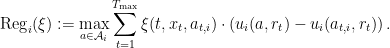We will model these guarantees as asking for no subsequence regret, which generalizes the notion of external regret to be measured over some subsequence $\xi: \{1, \ldots, T_\mathrm{max}\} \times \mathcal{X} \times \mathcal{A}_i \to [0, 1]$ , which may depend not only on $t$ and the past history, but also on any available external context (e.g., is it raining? Is there a Phillies game tonight?) and even on the agent’s own (as yet undecided) action (should I use I-76?). Given a subsequence function $\xi$ , we define an agent’s subsequence regret to be:

$\displaystyle \mathrm{Reg}_i(\xi) := \max_{a \in \mathcal{A}_i} \sum_{t=1}^{T_\mathrm{max}} \xi(t,x_t,a_{t,i}) \cdot \left(u_i(a, r_t) - u_i(a_{t, i}, r_t)\right).$

If there is only one subsequence the agent is interested in — or, for that matter, multiple non-overlapping subsequences — then as long as the subsequences are defined independently of the agent’s own actions, we could just run a separate copy of an off-the-shelf no-external-regret algorithm on every subsequence. This no longer makes sense for subsequences that depend on the agent’s action, since we would have now introduced a circularity. And naturally, the agent may simultaneously be interested in optimizing her regret over multiple overlapping subsequences: after all, rainy days, days when the Phillies are playing, and days when it seems to make sense to take I-76 are not mutually exclusive. So the question is: given a collection of subsequence functions $\xi_1,\xi_2, \ldots$ , can we make predictions that for every agent simultaneously promise low subsequence regret on all of these subsequences?

An application of this program: No subsequence regret for agents who best-respond to predictions
In any online combinatorial optimization setting with a set of agents $i \in \{1, \ldots, n\}$ , each of whom has utility function $u_i(\cdot, \cdot)$ and an arbitrary finite collection $\Xi_i$ of subsequences on which she desires to have no regret, we will now see how to use the $\mathcal{E}$ -unbiased prediction framework to provide, on all rounds $t$ , reward vector predictions $\hat{r}_t$ — the same prediction to all agents! — that simultaneously guarantee to each agent $i$ optimal regret on all her subsequences $\xi \in \Xi_i$ as long as she always simply best-responds to the predictions as if they were correct, i.e. $a_{t, i} = \mathrm{BR}(u_i, \hat{r}_t)$ .

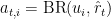
We’ll denote agent $i$ ‘s regret up to round $t$ on any subsequence $\xi \in \Xi_i$ as:

$\displaystyle \mathrm{Reg}_{t, i}(\xi) = \max_{a \in \mathcal{A}_i} \sum_{\tau=1}^{t} \xi(\tau, x_\tau, a_{\tau, i}) \cdot u_i(a, r_\tau) - \sum_{\tau=1}^{t} \xi(\tau, x_\tau, a_{\tau, i}) \cdot u_i(a_{\tau, i}, r_\tau).$
Let $\mathrm{len}_t(\xi) := \sum_{\tau=1}^{t} \xi(\tau, x_\tau, a_{\tau, i})$ denote the length of a subsequence $\xi$ by the end of round $t$ .

Theorem (No-Subsequence Regret for Downstream Agents in Online Combinatorial Optimization [NRRX23])
Consider an online combinatorial optimization problem with $d$ base elements $e \in \{1, \ldots, d\}$ , agents $i \in \{1, \ldots, n\}$ with respective utility functions $u_i(\cdot, \cdot)$ and subsequence collections $\Xi_i$ , and time horizon $T_\mathrm{max}$ . By appropriately instantiating our $\mathcal{E}$ -unbiased prediction framework, we can produce (randomized) reward vector predictions $\hat{r}_1, \ldots, \hat{r}_{T_\mathrm{max}}$ such that when the agents best-respond to them: $a_{t, i} = \mathrm{BR}(u_i, \hat{r}_t)$ — every agent $i$ obtains optimal expected regret on all of her subsequences at all rounds $t \leq T_\mathrm{max}$ (with the expectations taken over the randomness of our predictions):

$\displaystyle \mathop{\mathbb{E}}[\mathrm{Reg}_{t, i}(\xi)] = O \! \left( \!\! \sqrt{d \ln \left( \! d T_\mathrm{max} \! \sum_{i=1}^n \! |\Xi_i| \!\right) \! \cdot \! \mathop{\mathbb{E}}[\mathrm{len}_t(\xi)] } \! \right) \text{ for all } i, \xi \!\in\! \Xi_i, t \!\leq\! T_\mathrm{max}.$

Moreover, the algorithm is computationally efficient (poly-time in $d$ and in the total number $\sum_{i=1}^n |\Xi_i|$ of subsequences) so long as each agent has an efficient method for best-response computation (i.e., finding the $\mathop{\mathrm{argmax}}_{a \in \mathcal{A}_i} u_i(a, r)$ for any $r \in [-1, 1]^d$ ).

Proof
The event collection $\mathcal{E}_\mathrm{OCO}$ that implies the statement of our theorem will consist of the following $(d+1) \sum_{i=1}^n |\xi_i|$ events. For every agent $1 \leq i \leq n$ and every subsequence $\xi \in \Xi_i$ , $\mathcal{E}_\mathrm{OCO}$ will include:

An event $E_\xi$ that is active whenever the corresponding subsequence is active, defined for all $t$ as: $E_\xi(t, x_t, \hat{r}_t) = \xi(t, x_t, \mathrm{BR}(u_i, \hat{r}_t))$ ;
And, for every base element $e \in \{1, \ldots, d\}$ , an event $E_{\xi, e}$ that is active whenever the corresponding subsequence is active and when agent $i$ selects an action containing $e$ , defined for all $t$ as: $\displaystyle E_{\xi, e}(t, x_t, \hat{r}_t) = \xi(t, x_t, \mathrm{BR}(u_i, \hat{r}_t)) \cdot 1[e \in \mathrm{BR}(u_i, \hat{r}_t)]$ (where $1[e \in \mathrm{BR}(u_i, \hat{r}_t)]$ is the indicator of whether or not agent $i$ includes element $e$ in her selection when best-responding to prediction $\hat{r}_t$ ).

What does this event collection accomplish? Informally, it will guarantee that on every relevant subsequence for any agent $i$ , if agent $i$ adopts a predictions-to-actions policy $f \in \left\{ \{f^\mathrm{BR}_{u_i}\} \cup \{f_a\}_{a \in \mathcal{A}_i} \right\}$ , where $f^\mathrm{BR}_{u_i}(\cdot) \equiv \mathrm{BR}(u_i, \cdot)$ is the best-response policy and each $f_a(\cdot) \equiv a$ is a constant-action policy, then the total utility that $f$ will obtain “in reality” (i.e., based on the true realizations of the reward vectors $r_\tau$ ) will be almost equal to the total utility $f$ would have obtained if our predictions $\hat{r}_\tau$ were in fact the true reward vectors. Why is this useful? Because in our setting, subsequence regret measures the difference in the total utility of the best-response policy and of the best-performing constant-action policy over the subsequence, so the above would imply that the agent’s subsequence regret is almost the same as in the counterfactual world where our predictions were fully correct — which would be excellent and would imply the claim of our theorem, as the agent’s policy of best-responding to the predictions would by definition have optimal subsequence regret in that “alternate universe”.

To be more formal, let us fix $i, t, \xi \in \Xi_i$ , and start by showing the following two helper lemmas: one giving a guarantee on the total utility (on subsequence $\xi$ , up to round $t$ ) of the best-response policy, and the other doing the same for the benchmark, constant-action policies. For simplicity, we will ignore the error expressions and simply write $\approx$ to mean “up to an error term”; the precise subsequence regret bound we are claiming above can be easily read off from our generic $\mathcal{E}$ -unbiasedness guarantee. Also, once again for simplicity, we will omit the expectation signs ( $\mathbb{E}$ ) from the derivations below.

Helper Lemma 1: The unbiasedness of $\{\hat{r}_\tau\}_{\tau=1}^t$ conditional on $\{E_{\xi, e}\}_{e=1}^d$ implies that the total utility of the best-response policy $f^\mathrm{BR}_{u_i}(\cdot) \equiv \mathrm{BR}(u_i, \cdot)$ on subsequence $\xi$ up to round $t$ is (almost) the same no matter whether it’s measured relative to the actual rewards $r_\tau$ or relative to the predicted rewards $\hat{r}_\tau$ .

Proof of Helper Lemma 1: Recalling that $a_{t, i} = \mathrm{BR}(u_i, \hat{r}_t)$ , note the following (where the $\approx$ transition is by definition of $\hat{r}_\tau$ being unbiased on the events $E_{\xi, e}$ for all $e$ ):

$\displaystyle \sum_{\tau=1}^{t} \!\! \xi(\!\tau\!, x_\tau\!, a_{\tau, i}\!) \!\cdot\! u_i(a_{\tau, i}, r_\tau\!) \!=\!\! \sum_{\tau=1}^{t} \! \xi(\!\tau\!, x_\tau\!, a_{\tau, i}\!) \!\!\! \sum_{e \in a_{\tau, i}} \!\!\! r_{\tau, e} \!=\!\! \sum_{e=1}^d \! \sum_{\tau=1}^{t} \! \xi(\!\tau\!, x_\tau\!, a_{\tau, i}\!) \!\cdot\! 1\![e \!\in\! a_{\tau, i}] \!\cdot\! r_{\tau, e}$

$\displaystyle \!\!=\!\! \sum_{e = 1}^d \! \sum_{\tau=1}^{t} \! E_{\xi, e}(\tau, x_\tau, \hat{r}_\tau) \!\cdot r_{\tau, e} \!\!\approx\!\! \sum_{e = 1}^d \! \sum_{\tau=1}^{t} \! E_{\xi, e}(\tau, x_\tau, \hat{r}_\tau) \!\cdot \hat{r}_{\tau, e} \!\!=\!\! \sum_{\tau=1}^{t} \! \xi(\tau, x_\tau, a_{\tau, i}) \!\cdot u_i(a_{\tau, i}, \hat{r}_\tau).\hfill \mbox{\raggedright \rule{0.1in}{0.1in}}$

Helper Lemma 2: For every $a \in \mathcal{A}_i$ , the unbiasedness of $\{\hat{r}_\tau\}_{\tau=1}^t$ conditional on $E_\xi$ implies that the total utility of the constant-action policy $f_a(\cdot) \equiv a$ on subsequence $\xi$ up to round $t$ is (almost) the same no matter whether it’s measured relative to the actual rewards $r_\tau$ or relative to the predicted rewards $\hat{r}_\tau$ .

Proof of Helper Lemma 2: Note the following (where the $\approx$ transition is by definition of $\hat{r}_\tau$ being unbiased on the event $E_\xi$ ):

$\displaystyle \sum_{\tau=1}^{t} \xi(\tau, x_\tau, a_{\tau, i}) \cdot u_i(a, r_\tau) = \sum_{\tau=1}^{t} \xi(\tau, x_\tau, a_{\tau, i}) \sum_{e \in a} r_{\tau, e} = \sum_{e \in a} \sum_{\tau=1}^{t} \xi(\tau, x_\tau, a_{\tau, i}) \cdot r_{\tau, e}$

$\displaystyle \!=\! \sum_{e \in a} \! \sum_{\tau=1}^{t} \! E_\xi(\tau, x_\tau, \hat{r}_\tau) \cdot r_{\tau, e} \!\approx\! \sum_{e \in a} \! \sum_{\tau=1}^{t} \! E_\xi(\tau, x_\tau, \hat{r}_\tau) \cdot \hat{r}_{\tau, e} \!=\! \sum_{\tau=1}^{t} \! \xi(\tau, x_\tau, a_{\tau, i}) \cdot u_i(a, \hat{r}_\tau). \hfill \mbox{\raggedright \rule{0.1in}{0.1in}}$

Now, by combining the guarantees that we just obtained for the total utilities of the best-response and the constant-action policies, we can see that for any benchmark action $a \in \mathcal{A}_i$ :

$\displaystyle \sum_{\tau=1}^{t} \xi(\tau, x_\tau, a_{\tau, i}) \cdot u_i(a, r_\tau) - \sum_{\tau=1}^{t} \xi(\tau, x_\tau, a_{\tau, i}) \cdot u_i(a_{\tau, i}, r_\tau)$

$\displaystyle \approx \sum_{\tau=1}^{t} \xi(\tau, x_\tau, a_{\tau, i}) \cdot u_i(a, \hat{r}_\tau) - \sum_{\tau=1}^{t} \xi(\tau, x_\tau, a_{\tau, i}) \cdot u_i(a_{\tau, i}, \hat{r}_\tau).$

The right-hand side is $\leq 0$ since the actions $a_{\tau, i}$ are by definition best responses to the predictions $\hat{r}_\tau$ (in other words, the actions $a_{\tau, i}$ would have no regret to any policy on any subsequence, if our predictions $\hat{r}_\tau$ were the true reward vectors). Thus, the left-hand side is $\lessapprox 0$ for all benchmark actions $a \in \mathcal{A}_i$ .

But now, the definition of subsequence regret gives us the desired result (for all $i, \xi_i, t$ ):

$\displaystyle \mathrm{Reg}_{t, i} (\xi) \!=\! \max_{a \in \mathcal{A}_i} \! \left( \! \sum_{\tau=1}^{t} \! \xi(\tau, x_\tau, a_{\tau, i}\!) \!\cdot\! u_i(a, r_\tau) \!-\! \sum_{\tau=1}^{t} \xi(\tau, x_\tau, a_{\tau, i}) \!\cdot\! u_i(a_{\tau, i}, r_\tau) \!\right) \!\lessapprox\! 0. \hfill \mbox{\raggedright \rule{0.1in}{0.1in}}$

Note that this proof has exactly the same structure as our earlier proof that the best-response policy is optimal amongst all prediction-to-action policies for all utility functions if the forecasts are fully calibrated. The difference is that here, with a restricted class of benchmark policies (the constant-action policies, for every subsequence) and a restricted class of utility functions (the “combinatorial” utilities $u_i$ belonging to our specific agents $i \in \{1, \ldots, n\}$ ), we only needed for our predictions to be sufficient for estimating the total utility of the induced best-response policy and of all benchmark (constant-action) policies. And, as we just saw, this can be obtained with a much smaller set of conditioning events than required for full calibration.

How does this compare to previous approaches? The algorithm of [BM07] can be used by a single agent to obtain no subsequence regret guarantees, but in time that depends polynomially on the number of actions — which in this case is exponential in the dimension. By working in prediction space rather than action space, we are able to get two big wins. First, we can produce a single set of predictions that is simultaneously useful to many downstream agents. Second, we get exponential computational savings by taking advantage of the low-dimensional structure of utility functions in these settings. We could of course have obtained a qualitatively similar (though quantitatively much worse) guarantee from calibration; but by examining what we actually needed to get these guarantees, we found that in fact unbiasedness subject to a polynomial collection of events sufficed. This will turn out to be a common theme in many problems.

Outro

In this blog post, we have:

Discussed natural notions of calibration for predictive models;
Showed how acting as if a calibrated model’s predictions are correct is optimal amongst all prediction-to-decision policies, simultaneously for all downstream agents, no matter what their utility functions might be;
Hinted at the difficulty of (fully) calibrating high-dimensional predictions, and proposed a more flexible, decision-oriented notion of calibration that is much more efficient than full calibration in many natural decision pipelines;
Demonstrated an example of the power of decision-focused calibration in adversarial / strategic settings, by showing that it yields strong, flexible, and coordinated no-regret guarantees for one or more agents playing in an online combinatorial optimization game (e.g., a routing game) — similar to what full calibration would imply, but at only a tiny fraction of its computational and statistical cost.

In the next post, we will continue to explore applications of this decision-focused calibration methodology, applying it to solve two more challenging online problems:

Conformal prediction-style uncertainty quantification in online multiclass prediction; but without the need to choose a “conformity score”, and with stronger conditional guarantees;
Online model ensembles that simultaneously optimize many loss functions at once.

This will further reinforce our broader conceptual point:

Calibration, and uncertainty quantification more generally, should be done with an eye towards — and in the service of — concrete downstream applications of our model’s predictions.

Footnotes

There exist notions of calibration that avoid explicit bucketing [KF08, FH18, GKSZ22, BGHN23], but they will not be in our focus in this blog post. ↩︎
In what follows, we omit any arguments to $E$ that are implied or unused (like $x_t$ in non-contextual settings). ↩︎

References

[BGHN23] Jaroslaw Blasiok, Parikshit Gopalan, Lunjia Hu, and Preetum Nakkiran. A unifying theory of distance from calibration, 2023
[BM07] Avrim Blum and Yishay Mansour. From external to internal regret, 2007
[Daw82] A Philip Dawid. The well-calibrated Bayesian, 1982
[FH18] Dean P Foster and Sergiu Hart. Smooth calibration, leaky forecasts, finite recall, and Nash dynamics, 2018
[FV97] Dean P Foster and Rakesh V Vohra. Calibrated learning and correlated equilibrium, 1997
[FV98] Dean P Foster and Rakesh V Vohra. Asymptotic calibration, 1998
[FV99] Dean P Foster and Rakesh V Vohra. Regret in the on-line decision problem, 1999
[GHKRS23] Ira Globus-Harris, Declan Harrison, Michael Kearns, Aaron Roth, and Jessica Sorrell. Multicalibration as boosting for regression, 2023
[GJNPR22] Varun Gupta, Christopher Jung, Georgy Noarov, Mallesh M Pai, and Aaron Roth. Online multivalid learning: Means, moments, and prediction intervals, 2022
[GKSZ22] Parikshit Gopalan, Michael P Kim, Mihir A Singhal, and Shengjia Zhao. Low-degree multicalibration, 2022
[HJKRR18] Ursula Hebert-Johnson, Michael Kim, Omer Reingold, and Guy Rothblum. Multicalibration: Calibration for the (computationally-identifiable) masses, 2018
[HJZ23] Nika Haghtalab, Michael I Jordan, and Eric Zhao. A unifying perspective on multicalibration: Game dynamics for multi-objective learning, 2023
[KF08] Sham M Kakade and Dean P Foster. Deterministic calibration and Nash equilibrium, 2008
[KGZ19] Michael P Kim, Amirata Ghorbani, and James Zou. Multiaccuracy: Black-box post-processing for fairness in classification, 2019
[KV05] Adam Kalai and Santosh Vempala. Efficient algorithms for online decision problems, 2005
[NRRX23] Georgy Noarov, Ramya Ramalingam, Aaron Roth, and Stephan Xie. High-dimensional prediction for sequential decision making, 2023
[TW03] Eiji Takimoto and Manfred K Warmuth. Path kernels and multiplicative updates, 2003
[ZKSME21] Shengjia Zhao, Michael Kim, Roshni Sahoo, Tengyu Ma, and Stefano Ermon. Calibrating predictions to decisions: A novel approach to multi-class calibration, 2021

Share on Social Media